04 · June 2026
Numerical modelling of methane combustion
Three Python solvers for methane–air combustion, written from scratch without a kinetics library: adiabatic flame temperature (Newton–Raphson), 0D reactor ignition (RK4) and a 1D laminar flame profile (finite differences, Newton and the Thomas algorithm).
Specifications
- Mixture
- CH₄ + air, φ = 0.5 – 1.0
- Thermodynamics
- NASA-7 polynomials
- Kinetics
- single-step, Westbrook–Dryer
- Numerical methods
- Newton–Raphson · RK4 · FDM
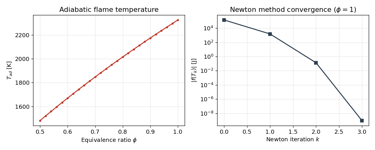
- Adiabatic flame temperature
- 2326 K (φ = 1)
- Apparent activation energy
- 175 kJ/mol
Project goal
I wrote three numerical methods for methane–air combustion from scratch, deliberately without a kinetics library such as Cantera. The combustion physics mattered less to me than the numerics: discretisation, convergence, and checking that the results can be trusted.
The global stoichiometric reaction:
CH₄ + 2 (O₂ + 3.76 N₂) → CO₂ + 2 H₂O + 7.52 N₂
Each part is a different kind of numerical problem: a nonlinear equation, a system of ordinary differential equations, and a partial differential equation.
| Part | Problem | Numerical method |
|---|---|---|
| 1 | Adiabatic flame temperature Tad(φ) | Newton–Raphson (nonlinear equation) |
| 2 | 0D reactor ignition: T(t), Y(t) | 4th-order Runge–Kutta (ODE system) |
| 3 | 1D laminar flame profile | finite differences, Newton and the Thomas algorithm (PDE) |
Methodology
Part 1: adiabatic flame temperature
I solve the mixture enthalpy balance for temperature with Newton–Raphson. The specific heat cp and enthalpy h come from 7-coefficient NASA polynomials in CHEMKIN format, with separate low- and high-temperature ranges.
For a stoichiometric mixture it converges in 3–4 iterations. The enthalpy residual drops from around 10⁵ J to below 10⁻⁸ J, quadratically, as theory says it should.
Part 2: 0D reactor
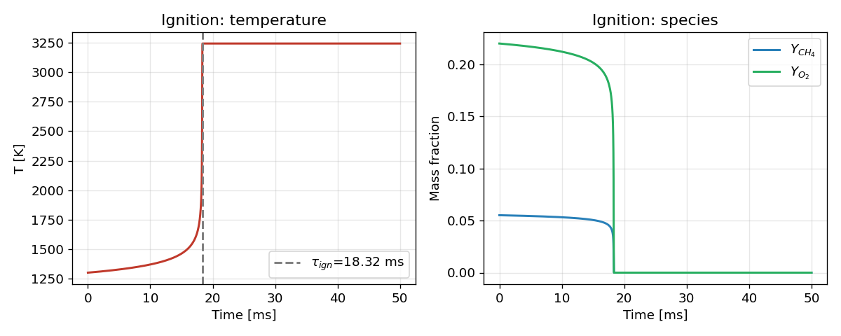
I model ignition in a homogeneous, adiabatic, constant-pressure reactor with single-step global Arrhenius kinetics after Westbrook and Dryer (1981). The reaction order is −0.3 in fuel and 1.3 in oxygen. I integrate the system in YCH₄, YO₂ and T with explicit 4th-order Runge–Kutta at a 1 µs step.
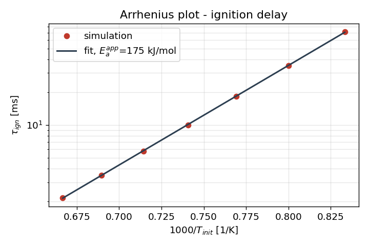
I computed the ignition delay for seven initial temperatures between 1200 and 1500 K, and got the apparent activation energy from a linear fit to the Arrhenius plot of ln(τ) against 1000/T.
Part 3: 1D laminar flame
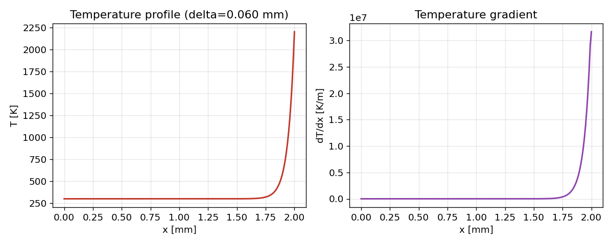
I solve the reaction–diffusion equation in the flame-front reference frame:
ρ cp Su dT/dx = d/dx (λ dT/dx) + q ω(T)
It is discretised with finite differences on a uniform grid: central differences for diffusion, upwind for convection. I solve the resulting nonlinear system with Newton–Raphson. The Jacobian is tridiagonal, so the Thomas algorithm handles each step in O(N) operations rather than the O(N³) of full Gaussian elimination.
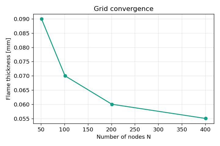
I checked the solution with a grid convergence study at 51, 101, 201 and 401 nodes.
Results
| Quantity | Result |
|---|---|
| Adiabatic flame temperature, φ = 1 | 2326 K |
| Newton iterations to convergence | 3–4 |
| Ignition delay, T₀ = 1300 K | 18.3 ms |
| Apparent activation energy | 175 kJ/mol |
| Flame front thickness, N = 201 | 0.060 mm |
The apparent activation energy came out at 175 kJ/mol, well below the 203 kJ/mol fed into the kinetic model. I expected that: the negative reaction order in fuel flattens how the ignition delay depends on temperature.
The grid study gave front thicknesses of 0.090 / 0.070 / 0.060 / 0.055 mm for 51, 101, 201 and 401 nodes. The value keeps falling and changes more slowly each time, but it hasn’t settled at 401 nodes. The flame front spans only a dozen or so nodes, so the result still depends on grid density.
Model limitations
The single-step mechanism ignores product dissociation, so the adiabatic flame temperature comes out higher than a full chemical equilibrium calculation would give. If I took the project further, I’d start with a multi-step mechanism, then add adaptive time stepping for the stiff system and solve for the laminar burning velocity Su as an eigenvalue of the boundary value problem.
Tools
Python 3 (NumPy, Matplotlib) · LaTeX
Results gallery